The Atomic Orbitals

Atom in a Box

Real-Time Visualization of the
Quantum-Mechanical Atomic Orbitals

What is Atom in a Box?

Atom in a Box is an application that aids in visualizing the Hydrogenic atomic orbitals, a prime and otherwise unwieldy example of quantum mechanics. Unlike other tools in this category, this program raytraces through a three-dimensional cloud density that represents the wavefunction's probability density and presents its results in real-time. The user interface is very interactive and provides a wide degree of flexibility.

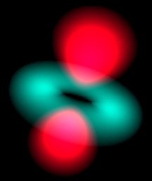
The app can display a wavefunction as a picture of a cloud or use color as phase. As of version 2, the Mac version of Atom in a Box can produce 2109 eigenstates up to the n=18 energy level, plus superpositions of up to 8 eigenstates of those 2109 eigenstates, allowing access to over 9 sextillion states! (9 with 21 zeros after it.)

Hint: After the eigenstates, a good next step are 2-eigenstate superpositions, of which there are 2,222,886 possible states, not counting the coefficients. You'd better get started!

How do I use Atom in a Box?

The bottom line is: PLAY WITH IT! Go ahead and try anything your heart desires. This document is meant for those who want more details about the program but is not required reading.

What is Atom in a Box for?

Think of an interactive exhibit at a science museum. If it can evoke imagination or fascination or stir inspiration or simply teach, then it's doing its work, maybe entertaining along the way.

Atom in a Box is like that. It gives a visual answer to: "What is an atom?" You can think of the atom as the building block of chemistry and everything we can see and touch. It's an important scientific concept that people have struggled with since the ancient Greeks. Now, if you could hold an atom, like a toy in your hands, this App shows what it might "look" like. If Atom in a Box can inspire fascination with science, then it has done its job. I think it looks cool too.

What is Quantum Mechanics?

One of the great advances in human knowledge of the twentieth century is the birth of the theory of Quantum mechanics. It has led to some of the most powerful technologies people use these days, including the little transistors that make up the computers you're using to read this. One of the mysteries it revealed was the structure of the atom. Classical mechanics could not properly explain the existence of the atom. Because there was nothing to stop electrons from spiralling in to the nucleus, it predicted that all atoms would immediately destroy themselves in a spectacular high-energy blast of radiation.

Well, that obviously doesn't happen. Quantum mechanics describes that the electron (and all of the universe for that matter) exists in any of a multitude of states. The particular physical situation determines what and how many states there are. Borrowing from some of the techniques in mathematics, physicists organize these states into a particular set of mathematically convenient states called "eigenstates". Eigenstates are good to use because what makes one eigenstate different from another usually has a physical meaning. They also can make an horribly difficult problem managable. These and other phenomena in Quantum mechanics predict that possiblities in physical phenomena have distinct separations (e.g., "quantum leaps") and that energy transport exists as indivisible packets, called "quanta". Hence the name: Quantum Mechanics.

What are Orbitals?

By applying these techniques to the hydrogen atom, physicists are able to precisely predict all of its properties. The electron eigenstates around the nucleus are called "orbitals", analogous to the orbit a planet occupies around a star. We find that these states do not allow the electron to crash into the nucleus, but instead find themselves in any combination of these orbital eigenstates. These orbitals' physical structure describe effects from how atoms bond to form compounds, magnetism, the size of atoms, the structure of crystals, to the structure of matter that we see around us.

Visualizing these states has been a challenge because the mathematics that describe the eigenfunctions are not simple and the states are a three-dimensional structures. The standard convention has the orbital eigenstates indexed by three interrelated integer indicies, called n, l, and m. Their range and interdependence comes out of the math in deriving the eigenstates from Quantum mechanics and electromagnetism. Special states, called eigenstates, have been found that, when properly summed together, can describe any allowed state of the electron bound to the nucleus. By definition, they cannot be written in terms of one another (i.e., they are said to be "orthogonal"). These eigenstates have their own unique labels.

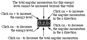
The first refers to the energy of the eigenstate, labeled by n. n can be any integer starting at one, the lowest energy level, then two, three, and so on for higher energies. Within an energy level, there are certain allowed distinct states of angular momentum which are identified by two integers, l and m. l can range from 0 to n-1 and identifies how much angular momentum the eigenstate has. m can range from -l to +l, identifying how much of that angular momentum is in the +z-direction. These three integers together uniquely identify every possible eigenstate, and are often written together in a Dirac ket: |n,l,m>. (For full details, look in a Quantum textbook (a good one is A Modern Approach to Quantum Mechanics by John S. Townsend), take a course, or seek out a physics professor.)

The number of eigenstates for energy level is the square of that energy level's quantum number n. So n=1 has one eigenstate, n=2 has four eigenstates, n=3 has nine, and so on.

For each eigenstate, Atom in a Box computes its wavefunction, a complex function of position. The magnitude squared of this function is plotted as brightness.

Version 1.x of the app computes up to n=7, the energy level for the highest energy electrons in the Uranium atom. Version 2.x of the Mac app computes, at run time, all the eigenstates up to n=18, so it can generate the complete description of up to 2109 eigenstates.

Changing the |n,l,m>'s

You can edit the |n,l,m> eigenstate by clicking it. You can step between these eigenstates by clicking on the + or - above and below the integers when available.

User interface details

Main view

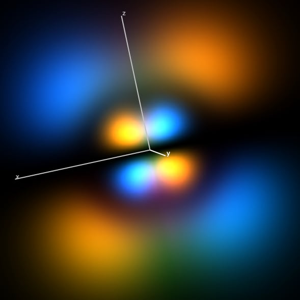
The primary display is the large square in the middle with the orbital in it. You can touch and drag your finger to rotate the orbital. Think as if you're poking your finger at it. If you're still moving it while you release, it will keep rotating. The small coordinate axes above the main display give a sense of reference to orient what you are seeing. Pressing space bar stops the motion. To make it easier to connect the orbital with its coordinate system, right-clicking makes large coordinate axes, centered on the orbital, appear.

View mode

The pop-up menu in the upper right of the menu toggles the View type. The Standard 3-D display mode shows the three-dimensional probability cloud as a two-dimensional image, like photographing a cloud in the sky.

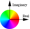
How color is mapped onto the complex plane

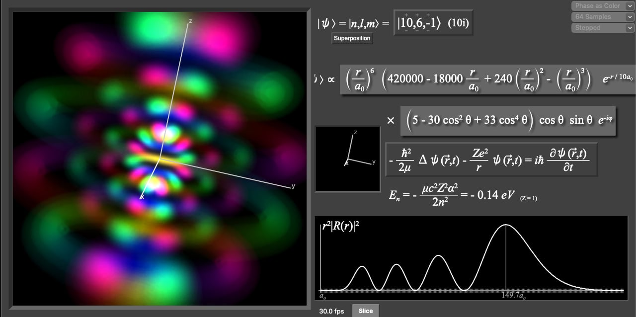
Using this popup menu toggles between Standard 3-D and Phase as Color. With Phase as Color, the phase of the wavefunction is translated into a hue of the cloud. The wavefunction is a complex valued function of position. Zero phase is translated into red, and increasing phase cycles through the color wheel, to yellow, to green, to cyan, to blue, to magenta, and back to red. Opposite phase corresponds to color complements, e.g., red and cyan represent opposite phases, yellow and blue are opposite, as are green and magenta.

Also with Phase as Color, you can see the time evolution of the wavefunction. Each eigenstate evolves in time at a rate related to its energy. For example, the states with m not equal to zero exhibit an electron flow around the z axis, like a small superconducting vortex.

The right of the orbital displays informative information relevant to the orbital, including:

1. The mathematical form of the wavefunction being displayed as a function of spherical coordinates r for radius, θ for angle from the +z axis, and φ for angle in the x-y plane starting from the +x axis.

2. Probability distribution of the electron as a function of radius r, with tick marks for every Bohr radius, a₀, a standard atomic length, and marked at the radius of maximum probability.

3. The energy of the electron in this wavefunction, along with that state's spectral label. Bound states have negative energy.

4. The three-dimensional time-independent Schrödinger equation, which is predicts all of these wavefunctions.

Samples menu

The code displays the wavefunctions by raytracing through the clouds and using a Simpson's rule integration technique to sum the contributions. As for all numerical integration, more samples usually mean higher accuracy (here a higher quality image), but more computation time spent, so the frame rate decreases (and the battery consumption increases). The Samples setting allows you to adjust this tradeoff.

Gamma menu

The Gamma setting allows you to adjust the probability density to brightness function. This adjustment makes it easier to see the structure of some wavefunctions. The cutoff gammas cut off the brightness if the density is below a certain value but do no adjustment above that value, and the stepped gammas translate the linear range of density into a stair-stepped set of brightness outputs, giving a more isosurfacish look. (The name originates in the "gamma table" of computer video hardware; video hardware gamma tables are used translate the linear R, G, and B, outputs into a nonlinear voltage output to the monitor to compensate for the nonlinear response of screen phosphor.)

Brightness (under the View menu)

After the wavefunction value is computed and before the Gamma table lookup, it is multipled by this Brightness factor. Raising this value will enhance low-probability details of the wavefunction, but often too much will obscure the brightest details. It is most useful with the various Gamma settings, above.

Sound (under Preferences)

Interprets the wavefunction with sound.

Atom in a Box Help

Opens a link to this online resource with additional information about Atom in a Box.

File menu

The Mac App can also save the orbital data into a file so you can save it for later or showing or sending to friends. We also provide a zip of several example orbitals that can be read with v2.0 or later of Atom in a Box. Remember that under new macOS, document-based apps like Atom in a Box will automatically save changes by default to the file, so changing any part of the orbital triggers a change to the "orbital document", which the system will automatically save to the file connected to that document. We advise being careful about saving backups. Fortunately our files are only 408 bytes each.

Note for those with files from v1.x of Atom in a Box: To have v2.0 of Atom in a Box read files written using v1.x of Atom in a Box, simply add the suffix ".orbital" to the file name to add the right filename extension. Unfortunately macOS 11.0 and later sets rules disallowing apps from recognizing the file types set in 20th-century Mac OS, but adding ".orbital" is how v2 of Atom in a Box can read two-decade-old files way back to 1999.

Privacy Policy

This developer does not collect any data from Atom in a Box or any data about users via Atom in a Box. Users may send files they save from the app to whomever they choose.

Behind the Scenes - How does this App do what it does?

The simplest brute force way of doing it, like how one might do it in Mathematica, would be to fill a large three-dimensional array of values using the mathematical solution of the wavefunction. Suppose you wanted a resolution of 256 x 256 x 256 in x, y, and z. Well, that's a little big, so you can probably interpolate from 128 x 128 x 128. That's about 2 million elements, each of which should require at least single-precision floating point numbers, which are 4 bytes big. Then that table would be 8 megabytes big. Of course, the wavefunction is complex, so that requires two floats per position, so that's 16 megabytes of data. And then you have to rotate your coordinates and raytrace through all of that. Even doing just an isosurface of that data can get slow without special hardware.

So, obviously, that's not it, because this entire application requires barely over a megabyte, much less than 16 megabytes. Another way might be to compute the wavefunction only when it is needed, so minimal data space is required. Well, you can have a look at the equations that the program displays. They have cosines, sines, and exponentials, all of which are nasty to numerically evaluate over and over again.

So what's the trick? In a programming tour de force for speed, this code utilizes lookup tables to an extreme. All operations more complicated than add and multiply are done using tables. That is, divides, square roots, exponentials, cosines, sines, arctangents, hue to RGB, etc. are all deep inside a combination of tables. And the tables are folded up in such a way so that all the tables used at any one time can fit inside the Level 1 cache onboard the processor.

So why did you do this?

The Mechanical Universe is a series of videotapes produced at Caltech that runs the gamut of first year undergraduate physics. It's an excellent source for visualizing and understanding basic concepts in physics. In one episode near the end, entitled "Atoms to Quarks", they show probability density clouds for the n=1 and 2 states, and stop at the |3,2,m> states. I loved it, but it all goes by very fast. The tapes date from the 1980's, so I'm sure they slowly computed all the images on some computer and dumped them to videotape frame by frame. That's the only time I remember seeing the orbitals plotted as probability clouds. All the other portrayals of orbitals I've seen are scatter plots and single isosurfaces, which really hide a great deal of the structure of orbitals, or, even worse, just the Ylm spherical harmonic functions from Mathematica without the radial dependence.

So I decided that I wanted to generate volumetric (i.e., clouds) plotting of the orbitals in real-time on my computer. My earliest attempts were on my //ci (68030 at 25 MHz) back in 1994, but there I only got as fast as one frame per minute (!) with no tables. My first PowerPC attempt with tables was in 1995, but it failed miserably (I wasn't using the tables correctly). Then in 1997, I resurrected the code and was a lot more careful and got Standard 3D and Red/Cyan 3D working and working fast. In January 1998, while I was at the American Association of Physics Teachers conference, I figured out how to quickly translate the phase of the wavefunction into color using tables in 1998.

Why the funky grayscale look?

Well, it's grayscale for two reasons: 1. Anything other than grayscale around the orbital is very distracting and hurts some people's eyes after a while. 2. It makes the color in the Phase as Color mode stand out more. So the theme I thought of here was like a piece of stereo equipment. In fact, Atom in a Box has used "Dark Mode" since 1997, decades before Apple added it to their OS. Atom in a Box has no "Light Mode".

And as for the funky part: From 1992 to 1994, I worked for a company, later known as MetaCreations, and was one of the two programmers who wrote Kai's Power Tools, a set of filters that plugged in to Adobe Photoshop for artists and advertisers. Besides doing neat things with images and being the first filter set with real-time previews, it had a very 3D-ish interactive user interface, coded by us two programmers (the other one still worked there until 2000) and designed by Kai Krause (he's done Yes album covers, among many things). Some users thought the UI was psychedelic (almost literally). So, I suppose my UI artistic style was influenced by my experience working with the people there, but perhaps I'm a little more reserved (and definitely more physics oriented).

Are there any easter eggs?

In the 2021 Mac version, no; it's not allowed on the App Store.

Thanks goes to Robert M. Zirpoli III and Professor Erica Carlson of the Physics and Astronomy Department at Purdue University for critiquing the Mac version of this program.

See the App Store for pricing and availability for your country.